Intro to Pandas
In the lessons covered in this course so far, we’ve covered the tools necessary to, given enough time and practice, perform most data analysis tasks that a scientist might want to do. However, like other things in Python, there are other tools that we can learn that can make that processes easier and more efficient. Pandas is data analysis toolbox created explicitly for this purpose.
Arguably the most useful feature of Pandas is the addition of useful data analysis data types, specifically the DataFrame, which collects data in a table like format with rows and columns with the ability to index and describe the data with a single data frame itself. DataFrames are a relatively complex data type and it is beyond the scope of this course to go too far down the rabbit hole in learning how to use and manipulate them. The goal here is to introduce them to you and provide some
basic working examples so that you can build on this knowledge in future courses and projects.
On nice feature of Pandas is that the tools are built to play nicely with numpy. This means that we can do things like convert parts of a DataFrame to a numpy array very quickly. Additionally, Pandas provides tools that enable us to quickly write data in a variety of formats, including CSV, HTML, and a various flavors of SQL.
Pandas Series
If you’ve been working with a recent version of Anaconda, then you should already have the ability to import pandas into you python session or programs. Before we get into working with the DataFrame type, let’s first take a look at the Pandas Series.
[1]:
import pandas as pd

mytemperatures = [20,15,18,36,35,19]
myseries = pd.Series(mytemperatures)
print(myseries)
0    20
1    15
2    18
3    36
4    35
5    19
dtype: int64
Right off, you should see there is a fundamental difference between the Series and the Array, as when I print the Series, there is some extra data that comes along with it. This is the “index” for each element in the series, and it is something that we can control.
[2]:
mytimes = [0,10,20,30,40,50]
myseries = pd.Series(mytemperatures,mytimes)
print(myseries)
0     20
10    15
20    18
30    36
40    35
50    19
dtype: int64
By specifying the index of each element, what I am able to do is attach meaningful information (metadata) to my data. For example, here I’ve assigned a measurement time to each of my temperature measurements. In this way, I can do things like query my data using the index that I’ve assigned:
[3]:
print(myseries.get(10))
15
instead of a index number. Let me be a little more realistic for this example and make use of the python date object from the datetime module. A date object is just what it sounds like, a way to quickly and easily add dates to your code.
[4]:
from datetime import date

year = 2019
month = 1
days = [1,3,5,7,9,11]
mydates = []

for d in days:
    mydates.append(date(year,month,d))

print(mydates)
[datetime.date(2019, 1, 1), datetime.date(2019, 1, 3), datetime.date(2019, 1, 5), datetime.date(2019, 1, 7), datetime.date(2019, 1, 9), datetime.date(2019, 1, 11)]
Now I have a list of dates that I can use to index my temperature data.
[5]:
myseries = pd.Series(mytemperatures,mydates)
print(myseries)
2019-01-01    20
2019-01-03    15
2019-01-05    18
2019-01-07    36
2019-01-09    35
2019-01-11    19
dtype: int64
Then if I want to grab the temperature for a specific day, I can use the date.
[6]:
adate = date(2019,1,7)
atemperature = myseries.get(adate)
print(atemperature)
36
Note that since the temperature series is indexed using a list of datetime date objects, then I need to use a date object when I “get” the data. In other words, I can’t simply index with a string like “2019-01-05”:
[7]:
strdate = "2019-01-05"
othertemperature = myseries.get(strdate)
print(othertemperature)
None
Pandas will allow you to query the Series but as you can see, the query returns a value of None since there is no index that matches such a string in my series.
You should think of the relationship between an index and the data in a series like you might think of a 2 column table in a spreadsheet program.
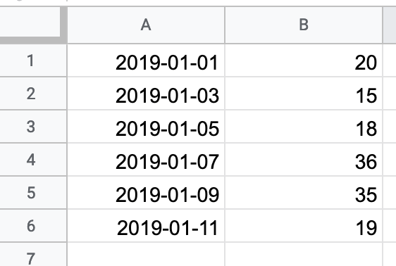
In this analogy, the number of rows in a spreadsheet corresponds to the number of elements in the series.
[8]:
print(len(myseries))
6
Pandas DataFrame
The Pandas Series is inherently a 1D data type with optional index labels. The DataFrame builds upon the idea of linking the data to the metadata to make it possible to store, query, and manipulate more complex 2D data. Let’s extend our example from above and replicate this table

using a DataFrame. I’ll start this process by adding data in to a numpy array. Normally, this data would be read from a file as in previous examples/exercises in this class. Here I’ll hard code it just to illustrate the point.
[9]:
import numpy as np
temperatureData = np.array([[20,16,18,30],\
                            [15,18,33,21],\
                            [18,28,19,13],\
                            [36,28,33,13],\
                            [35,28,28,17],\
                            [19,32,17,17]]\
                             )
print(temperatureData)
[[20 16 18 30]
 [15 18 33 21]
 [18 28 19 13]
 [36 28 33 13]
 [35 28 28 17]
 [19 32 17 17]]
At this point we have all the data in an array. Note that I used the “” or line continuation character which allows me to write the array using multiple lines. Now, we can create a DataFrame and populate it with this data as well as the information about the dates from above.
[10]:
columnNames = ["Site A","Site B","Site C","Site D"]
myDF = pd.DataFrame(temperatureData,index=mydates,columns=columnNames)
print(myDF)
            Site A  Site B  Site C  Site D
2019-01-01      20      16      18      30
2019-01-03      15      18      33      21
2019-01-05      18      28      19      13
2019-01-07      36      28      33      13
2019-01-09      35      28      28      17
2019-01-11      19      32      17      17
It looks like a proper table!
As I said, typically we’d read data from a file, so let’s see how to do that before moving on. As is often the case, I have some data in csv format. I’ve used python csv module in the past to read this data. Pandas also has a csv reader and it is even easier to use than what you’ve seen previously.
I will be using the file USC00200228.csv which contains rain, snowfall, snow depth, minimum, maximum, and observation temperature data each day for January - March 2020 in Ann Arbor, MI.
[11]:
file = "USC00200228.csv"
data = pd.read_csv(file)
In general, data files can have a lot of data, so I might not want to print the entire DataFrame here to examine it. A quick way to view a subset of the data is to use the head() and tail() methods, which print the beginning and end of the data frame respectively.
[12]:
print(data.head())
       STATION                 NAME        DATE  PRCP  SNOW  SNWD  TMAX  TMIN  \
0  USC00200228  ANN ARBOR SE, MI US  2020-01-01  0.05   0.8   2.0    30    24
1  USC00200228  ANN ARBOR SE, MI US  2020-01-02  0.00   0.0   1.0    37    23
2  USC00200228  ANN ARBOR SE, MI US  2020-01-03  0.00   0.0   0.0    47    30
3  USC00200228  ANN ARBOR SE, MI US  2020-01-04  0.00   0.0   0.0    43    33
4  USC00200228  ANN ARBOR SE, MI US  2020-01-05  0.02   0.2   0.0    35    29

   TOBS
0    24
1    30
2    40
3    33
4    29
[13]:
print(data.tail())
        STATION                 NAME        DATE  PRCP  SNOW  SNWD  TMAX  \
85  USC00200228  ANN ARBOR SE, MI US  2020-03-26  0.00   0.0   0.0    57
86  USC00200228  ANN ARBOR SE, MI US  2020-03-27  0.27   0.0   0.0    58
87  USC00200228  ANN ARBOR SE, MI US  2020-03-28  1.54   0.0   0.0    51
88  USC00200228  ANN ARBOR SE, MI US  2020-03-29  0.64   0.0   0.0    50
89  USC00200228  ANN ARBOR SE, MI US  2020-03-30  0.03   0.0   0.0    62

    TMIN  TOBS
85    27    44
86    38    38
87    36    42
88    42    50
89    40    40
Depending on the width of your screen, the data may be printed in 1 or 2 “blocks”. Ok, consider how awesome this is. With essentially one line of code, where we used pd.read_csv(), not only did we get all the data into a DataFrame, but that data is organized into rows and columns and the information about the columns names has already been added to the variable as well. In the “USC00200228.csv” file, all of the data is provided with quotes surrounding every entry which makes them look a
bit like strings. Let’s print the dtypes attribute of data to see what Pandas did with the data:
[14]:
print(data.dtypes)
STATION     object
NAME        object
DATE        object
PRCP       float64
SNOW       float64
SNWD       float64
TMAX         int64
TMIN         int64
TOBS         int64
dtype: object
So when we did the read, Pandas already figured out the appropriate data type of each column and stored the data appropriately. In other words, Pandas has handled all of the data entry with basically one line of code. We can now get a quick sense of the data using tools that you’ve seen before.
[15]:
print(len(data))
90
So we have 90 rows of data as expected as my file contained data for 3 months of observations.
[16]:
print(data.shape)
(90, 9)
The shape attribute tells us, again 90 rows, and 9 columns. We can quickly get the metadata, if there is any:
[17]:
print(data.columns.values)
print(data.index)
['STATION' 'NAME' 'DATE' 'PRCP' 'SNOW' 'SNWD' 'TMAX' 'TMIN' 'TOBS']
RangeIndex(start=0, stop=90, step=1)
Here we see the column headers are present as expected. The row index values are generic: here just a range from 0 to 90 incrementing by 1. This is expected since we didn’t tell Pandas how to index the data. read_csv() has an index keyword that we could have used like we did in the earlier examples.
Finally, with the names of the columns, it is easy to grab data by column!
[18]:
print(data['DATE'])
0     2020-01-01
1     2020-01-02
2     2020-01-03
3     2020-01-04
4     2020-01-05
         ...
85    2020-03-26
86    2020-03-27
87    2020-03-28
88    2020-03-29
89    2020-03-30
Name: DATE, Length: 90, dtype: object
[20]:
print(data[['NAME','PRCP']])
                   NAME  PRCP
0   ANN ARBOR SE, MI US  0.05
1   ANN ARBOR SE, MI US  0.00
2   ANN ARBOR SE, MI US  0.00
3   ANN ARBOR SE, MI US  0.00
4   ANN ARBOR SE, MI US  0.02
..                  ...   ...
85  ANN ARBOR SE, MI US  0.00
86  ANN ARBOR SE, MI US  0.27
87  ANN ARBOR SE, MI US  1.54
88  ANN ARBOR SE, MI US  0.64
89  ANN ARBOR SE, MI US  0.03

[90 rows x 2 columns]
Note the use of the double square brackets when printing multiple columns (e.g. I’m using a list of column names to “index” my dataframe.
At this point, you should start to see some of the benefits of Pandas series’ and data frames: they provide highly organized data structures that we can pull information from quickly and easily as well as tools to efficiently populate those data types. In the next lesson, we will further explore how we use these data types to do some quick analysis of our data.